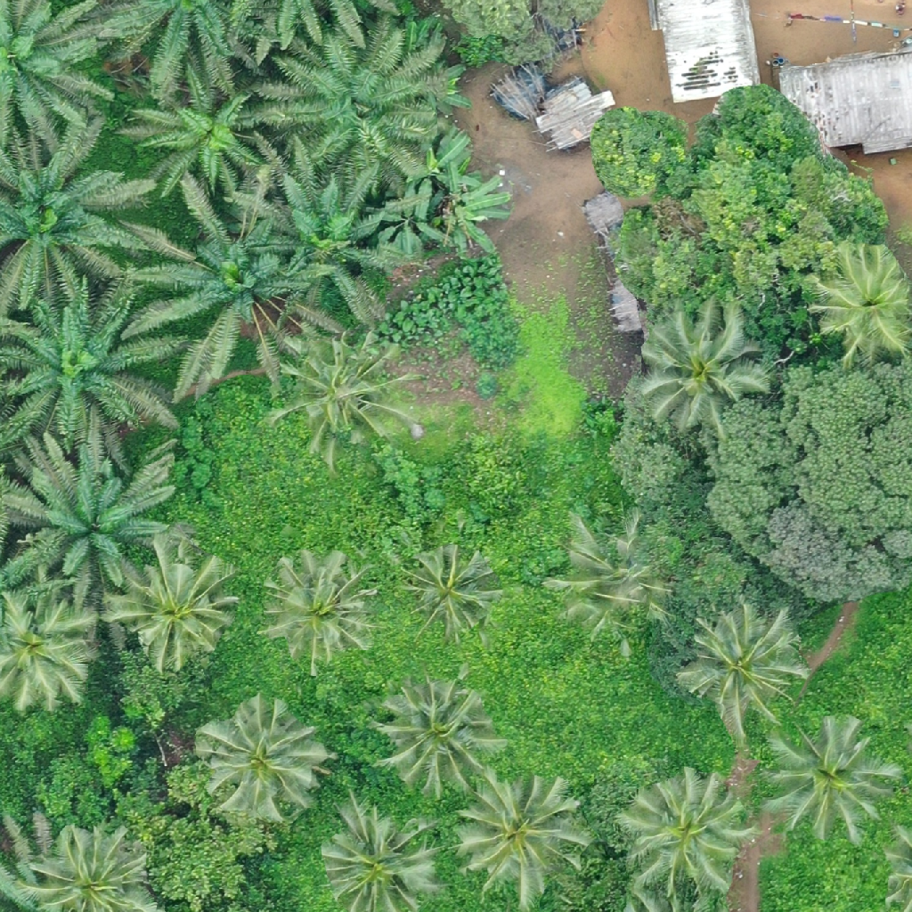
This article is a technical analysis of a project code submitted as part of an entry in the Zindi "Digital Africa Plantation Counting Challenge" [1]. The challenge aimed to develop a machine learning algorithm capable of accurately detecting and counting the number of palm oil trees in aerial images captured from drones. The code for the approach described here is available on Github [2].

The algorithm was trained on data consisting of a set of images, with labels corresponding to the number of palm trees in each image. The approach was applied to an unseen test set and those counts compared to ground truths on the Zindi platform.
At first, I was uncertain about how to tackle this task since it required counting and the training data lacked bounding boxes or segmentations, which are the types of data I've worked with in the past. As a result, I started researching density estimation and crowd counting techniques.
Density estimation is a computer vision technique used to estimate the distribution or density of objects in an image. In density estimation, the goal is to predict the likelihood of an object being present at each point in the image, rather than identifying or localising specific objects. One common application of density estimation is crowd counting, where the goal is to estimate the number of people in a crowded scene. Density estimation can also be used to estimate the distribution of other objects in an image, such as cars on a road or trees in a forest.
To perform density estimation, a density map is typically generated from the input image. A density map is a continuous 2D function that assigns a value to each pixel in the image, representing the expected density or likelihood of an object being present at that location. The density map can be generated using techniques such as kernel density estimation, where a Gaussian kernel is convolved with the image to estimate the density at each pixel.
Once the density map has been generated, it can be used as input to a machine learning model to predict the count or distribution of objects in the image. The model can be trained using labelled data that includes both the input images and their corresponding density maps, allowing it to learn to predict the object count or distribution from the density map. Some state-of-the-art crowd counting models are:
MCNN is one of the earliest CNN-based crowd counting models. It consists of multiple columns, each containing a different CNN, and a fusion layer that combines the outputs of these columns. MCNN is relatively simple and easy to implement, but it may not be as accurate as some of the newer models.
CSRNet is a more recent crowd counting model that uses a contextual pyramid CNN architecture. It has a hierarchical structure that captures both global and local information. CSRNet can handle high-density crowds and is known for its accuracy, but it may require more computational resources than MCNN.
SANet is another CNN-based crowd counting model that uses a scale aggregation network to estimate crowd density. It can capture multi-scale features and handle density variations in crowded scenes. SANet has shown promising results in challenging scenarios, such as scenes with occlusions and severe density variations.
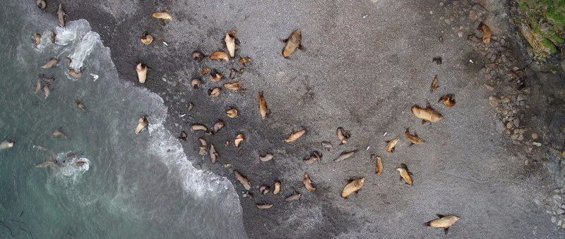
The NOAA Fisheries Steller Sea Lion Population Count Challenge [6] was a competition hosted on Kaggle with a similar aim to count sea lions in aerial imagery. The competition aimed to improve the accuracy and efficiency of population monitoring of Steller sea lions, an endangered species found in the western and northern coastal areas of North America.

The winning participant of this challenge used a Visual Geometry Group 16 (VGG16) [7] neural network architecture without the final layer, and added two fully connected (FC) layers with 1024 and 5 neurons respectively, with a linear output. They used stochastic gradient descent (SGD) as the optimisation algorithm and mean squared error (MSE) as the loss function.
Following a literature review, particularly the paper "Comparison of Deep Learning Methods for Detecting and Counting Sorghum Heads in UAV Imagery" [8], I opted for a similar approach to the Sea Lion counting challenge, but with the latest EfficientNet and ResNet models.
EfficientNet [9]: EfficientNet is a family of deep neural network architectures that were introduced in 2019. They use a compound scaling method to balance the number of parameters, Floating Point Operations Per Second (FLOPS), and accuracy. The EfficientNet architecture achieved state-of-the-art performance on the ImageNet classification task with significantly fewer parameters and computational cost than previous architectures.
ResNet [10]: ResNet is a deep residual neural network architecture that was introduced in 2015. It uses residual connections to enable the model to learn deeper representations of the input data. ResNet achieved state-of-the-art performance on the ImageNet classification task and has been widely used in various computer vision applications.
Overall, ResNet and EfficientNet have achieved better performance than VGG on various computer vision tasks. This review of ML competitions [11] in computer vision states that in 2022 EfficientNet was the most popular pre-trained model amongst competition winners, due to it's efficiency and it being less resource intensive.
Initially, I conducted experiments on Google Colab Notebooks to access GPUs. Later, I shifted to Vast.ai [12], which is a cloud-based platform that offers access to a distributed network of computers for running machine learning and deep learning models. To simplify the process of working on a remote GPU docker, I developed several scripts to install the necessary libraries and synchronize between the local and remote environments using rsync.
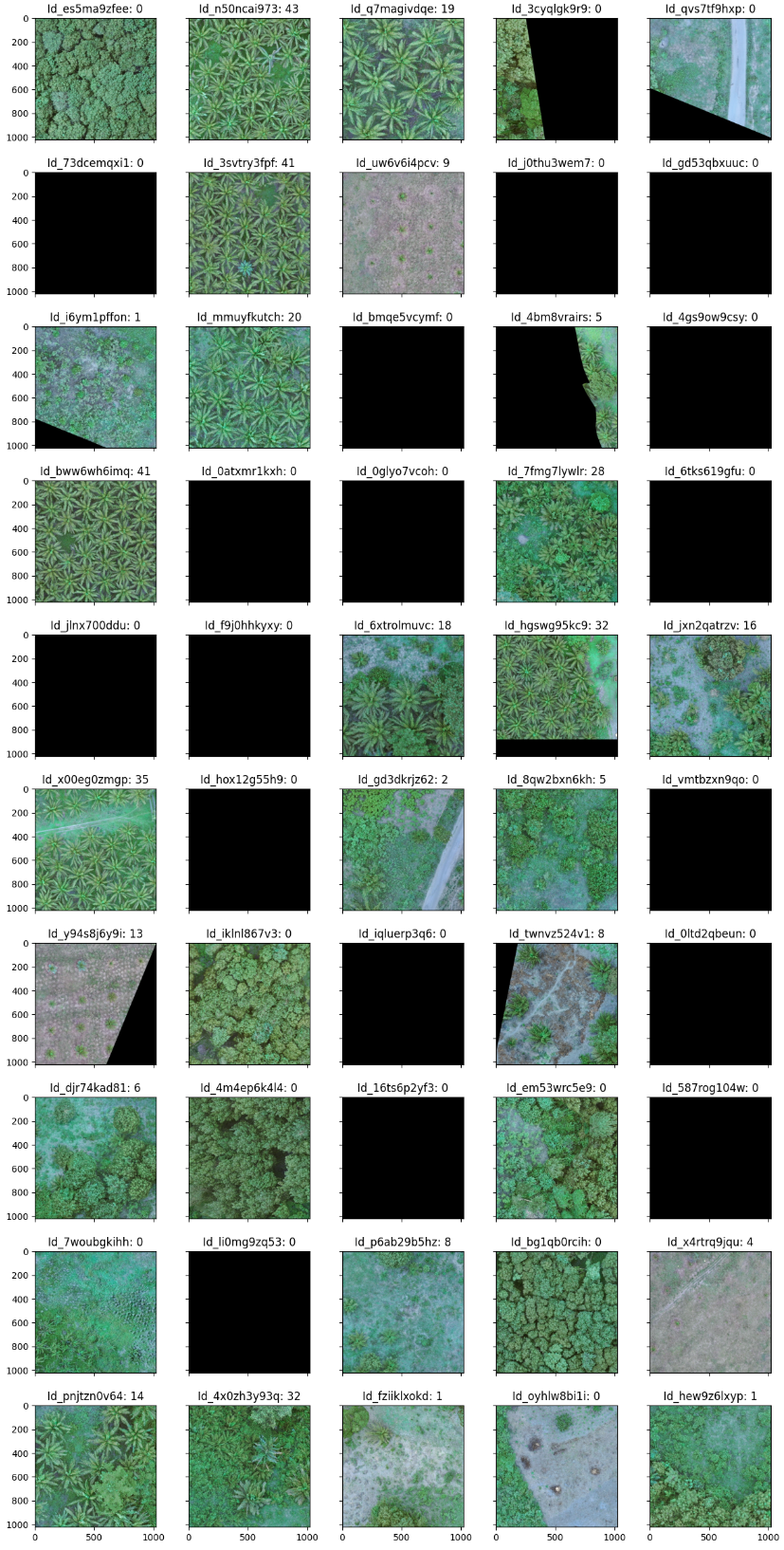
This data was collected using drones over 4 farms in Côte d'Ivoire in July and September 2022. There are 2002 images in train. There are 858 images in test.
A random sample of 50 images with their id, and target count from the training set can be seen below, representing the variation in the training set. Some images are blank and have a count of zero.

An initial exploratory data analysis (EDA) revealed that within the set of 2860 images, 807 images were completely empty (all pixels value 0).
Normalising data before using a CNN is an important step in preparing the data for training by scaling to standard range. Typically this range is between 0 and 1, or between -1 and 1, this re-scaling is achieved by subtracting the mean and dividing by the standard deviation of the input data.
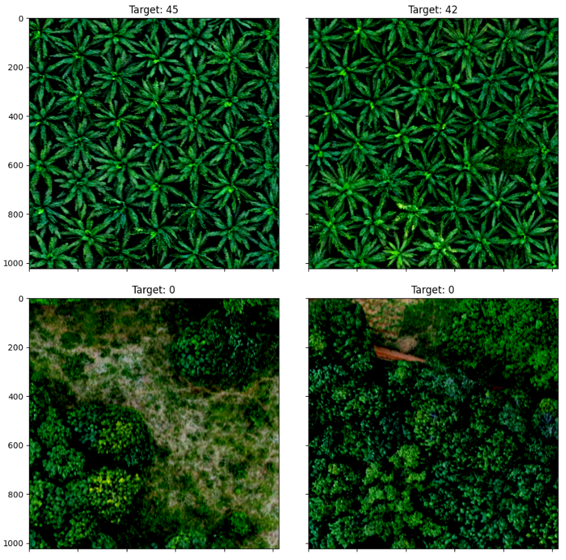
To determine the range to normalise I looped through all the images in the training data, excluding the empty images and obtained for each channel the mean values for each of the red, green and blue channels, as well as the standard deviations. The normalised images looked like this:

The idea behind data augmentation is to create new training examples by applying different transformations to the existing images in the training set, such as rotation, translation, scaling, flipping, and cropping. It is a popular technique in computer vision tasks, where large amounts of labeled data are required to train deep learning models effectively. These transformations change the appearance of the image while keeping the class label the same, and they help to make the model more robust to variations in the input data.
For this task I used transformations that would not lose information in the image that might affect the count, for example cropping. The augmentation pipeline I used for training was as follows.e:
The parameters used for example the blur kernel were customisable and stored in the params.yaml file.
In PyTorch the nn.Module is a base class that serves as the building block for creating neural networks. I used this to define and EfficientNetCounter and a ResNetCounter class. The nn.Module class provides methods for initialising the network parameters, defining the forward pass computation, and calculating gradients during back-propagation.
class EfficientNetCounter(nn.Module):
    """
    A PyTorch module for counting objects using EfficientNet.

    Args:
        params (dict): A dictionary containing the configuration parameters for the model.
            - model_name (str): The name of the EfficientNet model to use.

    Attributes:
        model (EfficientNet): The pre-trained EfficientNet model.
        fc (nn.Linear): The fully-connected layer for counting objects.
        relu (nn.ReLU): The activation function for the fully-connected layer.

    """
    def __init__(self, params=None):
        super(EfficientNetCounter, self).__init__()
        self.model = EfficientNet.from_pretrained(params.get("model_name"))
        self.fc = nn.Linear(1000, 1)
        self.relu = nn.ReLU()

    def forward(self, x):
        x = self.model(x)
        x = self.fc(x)
        return self.relu(x)
This code defines a PyTorch module called EfficientNetCounter that uses the pre-trained EfficientNet model to count objects in an image. The module takes a dictionary of configuration parameters params as input, which specifies the name of the EfficientNet model to use.
The __init__ method of the EfficientNetCounter class initialises the pre-trained EfficientNet model with the specified model_name from the params.yaml and adds a fully-connected layer fc with input size of 1000 and output size of 1. The output of this fully-connected layer is passed through a Rectified Linear Unit (ReLU) activation function relu.
class ResNetCounter(nn.Module):
    """
    A PyTorch module for counting objects using ResNet.

    Args:
        params (dict): A dictionary containing the configuration parameters for the model.
            - model_name (str): The name of the ResNet model to use.

    Attributes:
        model (nn.Sequential): The pre-trained ResNet model, with its final layers removed.
        fc1 (nn.Linear): The first fully-connected layer for counting objects.
        fc2 (nn.Linear): The second fully-connected layer for counting objects.

    """
    def __init__(self, params=None):
        super(ResNetCounter, self).__init__()
        self.model = getattr(models, params.get("model_name"))(pretrained=True)
        self.model = nn.Sequential(*list(self.model.children())[:-2])

        self.fc1 = nn.Linear(512*7*7, 256)
        nn.init.xavier_uniform_(self.fc1.weight)
        nn.init.zeros_(self.fc1.bias)
        self.fc2 = nn.Linear(256, 1)
        nn.init.xavier_uniform_(self.fc2.weight)
        nn.init.zeros_(self.fc2.bias)

    def forward(self, batch):
        x = self.model(batch)
        x = nn.Flatten()(x)
        x = self.fc1(x)
        x = self.fc2(x)
        x = nn.functional.relu(x)
        return x
The second architecture I experimented with used a pre-trained ResNet model to count objects in an image. The module takes a dictionary of configuration parameters params as input, which specifies the name of the ResNet model to use.
The __init__ method of the ResNetCounter class initializes the pre-trained ResNet model with the specified model_name and removes its final two layers. Then, two fully-connected layers fc1 and fc2 are added for counting objects. The first fully-connected layer has an input size of 51277 (output from the ResNet model) and output size of 256, while the second fully-connected layer has an input size of 256 and output size of 1. Xavier initialisation is used for the weights of both fully-connected layers, and their biases are initialized to zero.
The forward method defines the forward pass of the module. The input batch is passed through the pre-trained ResNet model, and the output is flattened using the nn.Flatten() function. The flattened output is then passed through the two fully-connected layers, and the resulting output is passed through a Rectified Linear Unit (ReLU) activation function before being returned.
With these two model architectures and the infrastructure for training I could use the params.yaml file to and scripts/run-remote.sh to experiment with different hyper-parameters for example:
normalize:
  rgb_means: [0.41210787, 0.50030631, 0.34875169]
  rgb_stds: [0.15202952, 0.15280726, 0.1288698]
transforms:
  resize: 380  # heigt and width are the same
  rescaler: false  # use the rescaler function to strech images
  jitter_brightness: [0.5, 1.5]
  jitter_contrast: 1
  jitter_saturation: [0.5, 1.5]
  jitter_hue: [-0.1, 0.1]
  blur_kernel: [1, 7]
  blur_sigma:  [0.1, 2]
  h_flip_probability: 0.5  # horizontal flip
  v_flip_probability: 0.5  # vertical flip
net:
  efficientnet:
    model_name: "efficientnet-b3"
    val_split: 0.15
    learning_rate: 0.0005 # 1e-3 # 1e-4
    batch_size: 67
    max_epochs: 50
    early_stopping_patience: 3
  resnet:
    model_name: "resnet34"
    val_split: 0.15
    learning_rate: 0.001 # 1e-3 # 1e-4
    batch_size: 80
    max_epochs: 40
    early_stopping_patience: 5
The output for each run was collected in a runs.csv. The best score was achieved using efficientnet-b3 and a batch size of 5.
| run | 20230331_140249 | 20230331_160035 | 20230403_154042 | 20230405_115823 |
|---|---|---|---|---|
| loss | 2.51 | 2.64 | 3.46 | 9.41 |
| model_name | efficientnet-b3 | efficientnet-b7 | resnet152 | resnet18 |
| learning_rate | 0.001 | 0.001 | 0.001 | 0.001 |
| batch_size | 5 | 5 | 20 | 200 |
| image_size | 1024 | 600 | 448 | 224 |
| image_rescaler | False | True | True | False |
| blur_kernel | [1, 9] | [1, 9] | [1, 5] | [1, 5] |
| blur_sigma | [0.1, 2] | [0.1, 2] | [0.1, 2] | [0.1, 2] |
| mem_usage | 20939 | 22193 | 18095 | 9440 |
| elapsed_time | 6099 | 8312 | 5187 | 2276 |
The columns are defined as follows:
run - Name of run constructed using run date, time, and model>loss - The validation loss achieved on the run.model_name - The pretrained model used.learning_rate - The learning rate as a float.batch_size - The number of images in a batch.image_size - The size of image used in neural network.image_rescaler - Whether images were rescaled as a boolean.blur_kernel - The data augmentation blur kernel used.blur_sigma - The data augmentation blur sigma value.mem_usage - The maximum memory usage from training the network.elapsed_time - The total training time in seconds.For each experiment, the logs, trained model and a csv of predictions is also generated.
Throughout this project, I gained valuable experience in running deep learning models with PyTorch on Vast.ai, and I believe this knowledge will serve as a useful template for tackling future computer vision challenges involving remote sensing data. Although I had hoped to implement various crowd estimation techniques, time constraints compelled me to prioritise writing reusable project infrastructure code that I can use again in future. Nonetheless, this project has been an enriching learning opportunity, and I look forward to applying this experience to future endeavours in the field of computer vision.
In addition to experimenting with more models I would like to improve the infrastructure using TensorBoard to better visualise model performance [12], and a library such as neptune for better keeping track of experiments [13]. It could also be helpful to use Grad-CAM (Gradient-weighted Class Activation Mapping) is a technique used in deep learning to visualise the regions of an input image that are important for a specific prediction made by a convolutional neural network (CNN). It computes a class activation map by using the gradients of the output of the CNN with respect to the feature maps of the final convolutional layer. This allows us to highlight the regions of the input image that are most relevant for the CNN's prediction, providing insight into how the network is making its decisions.
It has been a lot of fun to take part in this competition and thank you for Zindi and Digital Africa for hosting the competition and providing the data.
Zindi: Digital Africa Plantation Counting Challenge
↩github.com/williamgrimes/zindi_tree_counting_competition
↩Multi-function Convolutional Neural Networks for Improving Image Classification Performance
↩An effective modular approach for crowd counting in an image using convolutional neural networks
↩Scale Aggregation Network for Accurate and Efficient Crowd Counting
↩NOAA Fisheries Steller Sea Lion Population Count: Winning Solution
↩Very Deep Convolutional Networks for Large-Scale Image Recognition
↩Comparison of Deep Learning Methods for Detecting and Counting Sorghum Heads in UAV Imagery
↩Deep Residual Learning for Image Recognition.
↩ML Contests: The State of Competitive Machine Learning
↩Neptune: How to Keep Track of Experiments in PyTorch
↩